Space Apps Challenge 2018

Challenges:
1. Transportation mode
2. Power source
3. Autonomy including the mapping algorithm and the path planning algorithm

Resources:
1. http://bdml.stanford.edu/Main/HomePage
2. https://www.dexterindustries.com/gopigo3/
3. N. Sariff and N. Buniyamin, "An Overview of Autonomous Mobile Robot Path Planning Algorithms", Buniyamin
4th Student Conference on Research and Development (Scored 2006), June 2006
4. AK Guruji, "Time-efficient A* Algorithm for Robot Path Planning", ScienceDirect, 2016
5. Solidworks 2014
6. Claudiu Popirlan and Mihai Dupac, "An Optimal Path Algorithm for Autonomous Searching Robots", Annals of University of Craiova, Math. Comp. Sci. Ser., Volume 36(1), 2009

Impactof MMOD on Spaceships:

Spacecraftin low earth orbit (LEO) experience a variety of hazards includingexposure to micrometeoroids and orbital debris (MMOD). Average impactspeeds for orbital debris on spacecraft in LEO are 9 to 10 km/s, and20 km/s for micrometeoroids. Due to their high speeds, MMOD can causeconsiderable impact damage to sensitive spacecraft surfaces such aswindows, structural elements, electronic boxes, solar arrays,radiators, thermal protection system (TPS) materials coveringcrew/cargo return vehicles, as well as crew modules. Prolongedexposure to the on-orbit MMOD environment can potentially compromisethe TPS covering return vehicles such as the future crewed vehiclesexpected to visit and remain for a half-year or longer at theInternational Space Station (ISS). However, determination of MMODimpact damage to the TPS on crew/cargo return vehicles, or damage toother orbiting spacecraft currently requires visual inspection.

Withan estimated more than 100 million pieces of orbital debris measuringsmaller than one centimeter currently in Earth’s orbit, they can betoo small to track, but many are large enough to cause damage tooperational spacecraft. Objects larger than 3 mm are monitored fromthe ground.

Orbitaldebris as small as .3mm may pose a danger to human spaceflight androbotic missions. “Debris this small has the potential to damageexposed thermal protection systems, spacesuits, windows andunshielded sensitive equipment,”

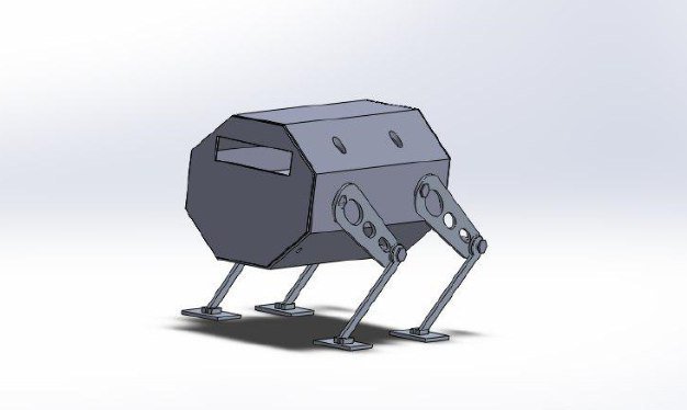
Designby Nature (Buckbeak Robot):

• Design a robot that simulatesthe “Gecko combined with dog” to create a trajectory of afree-flyer.
• The robot design is inspiredby nature, mimicking the adhesion of theGecko , the pacing of thedog and the transportation way of the mouse.
  Write a programfor this trajectory with Python.
  Decide on the shape of thefree-flyer, its energy source, and its technique for inspecting thesurface of the spacecraft including the signal type and its sensors(Including proximity sensors and edge sensors).
  A detailedapplicable design protocol of the building blocks of the free-flyerand its theory of operation: how it maintains its autonomy, whattypes of signals it uses and how they are processed, how itmaintains its safety and sustainability, etc.
• Model a design of the robotwith SolidWorks.

What will our idea change:

- Save crew time.

- Achievable autonomyalgorithm.

- Easier to further developdue to the GoPiGo front-end interface.

Theobjective of the solution:

• Detect the impact of the MMODon the body of the spaceship; so that we can avoid futurecatastrophes due to the resulting damage.
• Saves time and spares lots ofefforts; thanks to the robot autonomy.
• Simplify the control of therobot; because of the uncomplicated Python coding.

Componentsof the robot:

• Proximity Sensor:

A proximity sensor is anelectronic sensor that can detect the presence of objects within itsvicinity without any actual physical contact. In order to senseobjects, the proximity sensor radiates or emits a beam ofelectromagnetic radiation, usually in the form of infrared light, andsenses the reflection in order to determine the object's proximity ordistance from the sensor.
two sensors are needed for the robotdesign.

Type:CapacitiveSensors:Detection of metallic and non-metallic objects (Liquids, plastics,woods).

• RaspberryPi Camera:

Thecamera is adjustable one that is headed down to inspect thespacecraft body surface. The camera is adjacentto a proximity sensor, also there's another proximity sensorlocalized below it. Oncethe proximity sensor detects and impact; it turns the camera on. Thisway, the camera provides detailed information about the crack and itsposition.

• Basematerial :

Aluminium2018 Alloy

Advantages:

• Heattreatable wrought alloy.
• It is ahigh strength, age hardening, forging alloy.
• Copperis the chief alloying element.

• Externalbody:

Aluminium3003 Alloy

Advantages:

• Light.
• Highductility and corrosion resistance.
• Moderatestrength and good corrosion resistance.
• Thestrength of this alloy can be increased by cold working.
• Widelyused in space.
• gavebetter peroformance than other candidiates in MMOD hypervelocityimpact testing performed in Johnson Space Center.

• GoPiGo3Board:

TheGoPiGo3 is stacked with the Raspberry Pi withoutthe need for any other connections.

All themotor control and sensor I/O on the GoPiGo is done by an ATMEGA328microcontroller on the GoPiGo. The microcontroller acts as aninterpreter between the Raspberry Pi and the GoPiGo. It sends,receives, and executes commands sent by the RaspberryPi. Shortly, theGoPiGo3 board controls the body, sensors and motors all over therobot.

• EDIMAX- Wireless Adapters:

Establishesa Wi-Fi connection between the space shuttle and the robot. It uses alocal network.

• IRSensor:

Itprovides a wider angle for detection. Two sensors are needed for therobot design.

• Servomotor:

Thirteenmotors are needed for the robot design.

Type:MG995 – Torque 13.5 Kg.Cm, 0.16/60 degrees.

• Batteries:

3.7-kilowatt-hour lithium-ionbattery pack.

- Legs:

Adhesive legs made ofPolydimethylsiloxane(PDMS), fabricatedat Stanford Nanofabrication Facility.

Codes:

(1)

"""Extended Kalman Filter (EKF) Localization Sample Code.

Kalman filtering, also known as linear quadratic estimation (LQE), is an algorithm that uses a series of measurements observed over time, containing statistical noise and other inaccuracies, and produces estimates of unknown variables that tend to be more accurate than those based on a single measurement alone, by estimating a joint probability distribution over the variables for each timeframe"""

import numpy as np

import math

import matplotlib.pyplot as plt

# Estimation parameter of EKF

Q = np.diag([0.1, 0.1, math.radians(1.0), 1.0])**2

R = np.diag([1.0, math.radians(40.0)])**2

# Simulation parameter

Qsim = np.diag([0.5, 0.5])**2

Rsim = np.diag([1.0, math.radians(30.0)])**2

DT = 0.1 # time tick [s]

SIM_TIME = 50.0 # simulation time [s]

show_animation = True

def calc_input():

v = 1.0 # [m/s]

yawrate = 0.1 # [rad/s]

u = np.matrix([v, yawrate]).T

return u

def observation(xTrue, xd, u):

xTrue = motion_model(xTrue, u)

# add noise to gps x-y

zx = xTrue[0, 0] + np.random.randn() * Qsim[0, 0]

zy = xTrue[1, 0] + np.random.randn() * Qsim[1, 1]

z = np.matrix([zx, zy])

# add noise to input

ud1 = u[0, 0] + np.random.randn() * Rsim[0, 0]

ud2 = u[1, 0] + np.random.randn() * Rsim[1, 1]

ud = np.matrix([ud1, ud2]).T

xd = motion_model(xd, ud)

return xTrue, z, xd, ud

def motion_model(x, u):

F = np.matrix([[1.0, 0, 0, 0],

[0, 1.0, 0, 0],

[0, 0, 1.0, 0],

[0, 0, 0, 0]])

B = np.matrix([[DT * math.cos(x[2, 0]), 0],

[DT * math.sin(x[2, 0]), 0],

[0.0, DT],

[1.0, 0.0]])

x = F * x + B * u

return x

def observation_model(x):

# Observation Model

H = np.matrix([

[1, 0, 0, 0],

[0, 1, 0, 0]

])

z = H * x

return z

def jacobF(x, u):

"""

Jacobian of Motion Model

motion model

x_{t+1} = x_t+v*dt*cos(yaw)

y_{t+1} = y_t+v*dt*sin(yaw)

yaw_{t+1} = yaw_t+omega*dt

v_{t+1} = v{t}

so

dx/dyaw = -v*dt*sin(yaw)

dx/dv = dt*cos(yaw)

dy/dyaw = v*dt*cos(yaw)

dy/dv = dt*sin(yaw)

"""

yaw = x[2, 0]

v = u[0, 0]

jF = np.matrix([

[1.0, 0.0, -DT * v * math.sin(yaw), DT * math.cos(yaw)],

[0.0, 1.0, DT * v * math.cos(yaw), DT * math.sin(yaw)],

[0.0, 0.0, 1.0, 0.0],

[0.0, 0.0, 0.0, 1.0]])

return jF

def jacobH(x):

# Jacobian of Observation Model

jH = np.matrix([

[1, 0, 0, 0],

[0, 1, 0, 0]

])

return jH

def ekf_estimation(xEst, PEst, z, u):

# Predict

xPred = motion_model(xEst, u)

jF = jacobF(xPred, u)

PPred = jF * PEst * jF.T + Q

# Update

jH = jacobH(xPred)

zPred = observation_model(xPred)

y = z.T - zPred

S = jH * PPred * jH.T + R

K = PPred * jH.T * np.linalg.inv(S)

xEst = xPred + K * y

PEst = (np.eye(len(xEst)) - K * jH) * PPred

return xEst, PEst

def plot_covariance_ellipse(xEst, PEst):

Pxy = PEst[0:2, 0:2]

eigval, eigvec = np.linalg.eig(Pxy)

if eigval[0] >= eigval[1]:

bigind = 0

smallind = 1

else:

bigind = 1

smallind = 0

t = np.arange(0, 2 * math.pi + 0.1, 0.1)

a = math.sqrt(eigval[bigind])

b = math.sqrt(eigval[smallind])

x = [a * math.cos(it) for it in t]

y = [b * math.sin(it) for it in t]

angle = math.atan2(eigvec[bigind, 1], eigvec[bigind, 0])

R = np.matrix([[math.cos(angle), math.sin(angle)],

[-math.sin(angle), math.cos(angle)]])

fx = R * np.matrix([x, y])

px = np.array(fx[0, :] + xEst[0, 0]).flatten()

py = np.array(fx[1, :] + xEst[1, 0]).flatten()

plt.plot(px, py, "--r")

def main():

print(__file__ + " start!!")

time = 0.0

# State Vector [x y yaw v]'

xEst = np.matrix(np.zeros((4, 1)))

xTrue = np.matrix(np.zeros((4, 1)))

PEst = np.eye(4)

xDR = np.matrix(np.zeros((4, 1))) # Dead reckoning

# history

hxEst = xEst

hxTrue = xTrue

hxDR = xTrue

hz = np.zeros((1, 2))

while SIM_TIME >= time:

time += DT

u = calc_input()

xTrue, z, xDR, ud = observation(xTrue, xDR, u)

xEst, PEst = ekf_estimation(xEst, PEst, z, ud)

# store data history

hxEst = np.hstack((hxEst, xEst))

hxDR = np.hstack((hxDR, xDR))

hxTrue = np.hstack((hxTrue, xTrue))

hz = np.vstack((hz, z))

if show_animation:

plt.cla()

plt.plot(hz[:, 0], hz[:, 1], ".g")

plt.plot(np.array(hxTrue[0, :]).flatten(),

np.array(hxTrue[1, :]).flatten(), "-b")

plt.plot(np.array(hxDR[0, :]).flatten(),

np.array(hxDR[1, :]).flatten(), "-k")

plt.plot(np.array(hxEst[0, :]).flatten(),

np.array(hxEst[1, :]).flatten(), "-r")

plot_covariance_ellipse(xEst, PEst)

plt.axis("equal")

plt.grid(True)

plt.pause(0.001)

if __name__ == '__main__':

main()

(2)

"""2D Gaussian Grid Map Sample Code.

As the robot is small-sized reltive to the spacecraft's surface, it can view it as a 2D. A more efficient approach, however, would be to make a spacecraft-specific 3D grid map. Because this is just a proof-of-concept code, we chose to model a perfect 2D surface. Yet, this model, as it is, makes the robot most perfect for sufficiently large space structures."""

import math

import numpy as np

import matplotlib.pyplot as plt

from scipy.stats import norm

EXTEND_AREA = 10.0 # [m] grid map extention length

show_animation = True

def generate_gaussian_grid_map(ox, oy, xyreso, std):

minx, miny, maxx, maxy, xw, yw = calc_grid_map_config(ox, oy, xyreso)

gmap = [[0.0 for i in range(yw)] for i in range(xw)]

for ix in range(xw):

for iy in range(yw):

x = ix * xyreso + minx

y = iy * xyreso + miny

# Search minimum distance

mindis = float("inf")

for (iox, ioy) in zip(ox, oy):

d = math.sqrt((iox - x)**2 + (ioy - y)**2)

if mindis >= d:

mindis = d

pdf = (1.0 - norm.cdf(mindis, 0.0, std))

gmap[ix][iy] = pdf

return gmap, minx, maxx, miny, maxy

def calc_grid_map_config(ox, oy, xyreso):

minx = round(min(ox) - EXTEND_AREA / 2.0)

miny = round(min(oy) - EXTEND_AREA / 2.0)

maxx = round(max(ox) + EXTEND_AREA / 2.0)

maxy = round(max(oy) + EXTEND_AREA / 2.0)

xw = int(round((maxx - minx) / xyreso))

yw = int(round((maxy - miny) / xyreso))

return minx, miny, maxx, maxy, xw, yw

def draw_heatmap(data, minx, maxx, miny, maxy, xyreso):

x, y = np.mgrid[slice(minx - xyreso / 2.0, maxx + xyreso / 2.0, xyreso),

slice(miny - xyreso / 2.0, maxy + xyreso / 2.0, xyreso)]

plt.pcolor(x, y, data, vmax=1.0, cmap=plt.cm.Blues)

plt.axis("equal")

def main():

print(__file__ + " start!!")

xyreso = 0.5 # xy grid resolution

STD = 5.0 # standard diviation for gaussian distribution

for i in range(5):

ox = (np.random.rand(4) - 0.5) * 10.0

oy = (np.random.rand(4) - 0.5) * 10.0

gmap, minx, maxx, miny, maxy = generate_gaussian_grid_map(

ox, oy, xyreso, STD)

if show_animation:

plt.cla()

draw_heatmap(gmap, minx, maxx, miny, maxy, xyreso)

plt.plot(ox, oy, "xr")

plt.plot(0.0, 0.0, "ob")

plt.pause(1.0)

if __name__ == '__main__':

main()

(3)

"""Sample Code: A* Algorithm for Path Planning.

We chose A* algorithm becuase it is the most accurate although it does not necessarily generate the optimal path, but in our application we want the robot to walk as much as possible, and trace his path accurately."""

import matplotlib.pyplot as plt

import math

show_animation = True

class Node:

def __init__(self, x, y, cost, pind):

self.x = x

self.y = y

self.cost = cost

self.pind = pind

def __str__(self):

return str(self.x) + "," + str(self.y) + "," + str(self.cost) + "," + str(self.pind)

def calc_fianl_path(ngoal, closedset, reso):

# generate final course

rx, ry = [ngoal.x * reso], [ngoal.y * reso]

pind = ngoal.pind

while pind != -1:

n = closedset[pind]

rx.append(n.x * reso)

ry.append(n.y * reso)

pind = n.pind

return rx, ry

def a_star_planning(sx, sy, gx, gy, ox, oy, reso, rr):

"""

gx: goal x position [m]

gx: goal x position [m]

ox: x position list of Obstacles [m]

oy: y position list of Obstacles [m]

reso: grid resolution [m]

rr: robot radius[m]

"""

nstart = Node(round(sx / reso), round(sy / reso), 0.0, -1)

ngoal = Node(round(gx / reso), round(gy / reso), 0.0, -1)

ox = [iox / reso for iox in ox]

oy = [ioy / reso for ioy in oy]

obmap, minx, miny, maxx, maxy, xw, yw = calc_obstacle_map(ox, oy, reso, rr)

motion = get_motion_model()

openset, closedset = dict(), dict()

openset[calc_index(nstart, xw, minx, miny)] = nstart

while 1:

c_id = min(

openset, key=lambda o: openset[o].cost + calc_heuristic(ngoal, openset[o]))

current = openset[c_id]

# show graph

if show_animation:

plt.plot(current.x * reso, current.y * reso, "xc")

if len(closedset.keys()) % 10 == 0:

plt.pause(0.001)

if current.x == ngoal.x and current.y == ngoal.y:

print("Find goal")

ngoal.pind = current.pind

ngoal.cost = current.cost

break

# Remove the item from the open set

del openset[c_id]

# Add it to the closed set

closedset[c_id] = current

# expand search grid based on motion model

for i in range(len(motion)):

node = Node(current.x + motion[i][0],

current.y + motion[i][1],

current.cost + motion[i][2], c_id)

n_id = calc_index(node, xw, minx, miny)

if n_id in closedset:

continue

if not verify_node(node, obmap, minx, miny, maxx, maxy):

continue

if n_id not in openset:

openset[n_id] = node # Discover a new node

else:

if openset[n_id].cost >= node.cost:

# This path is the best until now. record it!

openset[n_id] = node

rx, ry = calc_fianl_path(ngoal, closedset, reso)

return rx, ry

def calc_heuristic(n1, n2):

w = 1.0 # weight of heuristic

d = w * math.sqrt((n1.x - n2.x)**2 + (n1.y - n2.y)**2)

return d

def verify_node(node, obmap, minx, miny, maxx, maxy):

if node.x < minx:

return False

elif node.y < miny:

return False

elif node.x >= maxx:

return False

elif node.y >= maxy:

return False

if obmap[node.x][node.y]:

return False

return True

def calc_obstacle_map(ox, oy, reso, vr):

minx = round(min(ox))

miny = round(min(oy))

maxx = round(max(ox))

maxy = round(max(oy))

# print("minx:", minx)

# print("miny:", miny)

# print("maxx:", maxx)

# print("maxy:", maxy)

xwidth = round(maxx - minx)

ywidth = round(maxy - miny)

# print("xwidth:", xwidth)

# print("ywidth:", ywidth)

# obstacle map generation

obmap = [[False for i in range(xwidth)] for i in range(ywidth)]

for ix in range(xwidth):

x = ix + minx

for iy in range(ywidth):

y = iy + miny

# print(x, y)

for iox, ioy in zip(ox, oy):

d = math.sqrt((iox - x)**2 + (ioy - y)**2)

if d <= vr / reso:

obmap[ix][iy] = True

break

return obmap, minx, miny, maxx, maxy, xwidth, ywidth

def calc_index(node, xwidth, xmin, ymin):

return (node.y - ymin) * xwidth + (node.x - xmin)

def get_motion_model():

# dx, dy, cost

motion = [[1, 0, 1],

[0, 1, 1],

[-1, 0, 1],

[0, -1, 1],

[-1, -1, math.sqrt(2)],

[-1, 1, math.sqrt(2)],

[1, -1, math.sqrt(2)],

[1, 1, math.sqrt(2)]]

return motion

def main():

print(__file__ + " start!!")

# start and goal position

sx = 10.0 # [m]

sy = 10.0 # [m]

gx = 50.0 # [m]

gy = 50.0 # [m]

grid_size = 1.0 # [m]

robot_size = 1.0 # [m]

ox, oy = [], []

for i in range(60):

ox.append(i)

oy.append(0.0)

for i in range(60):

ox.append(60.0)

oy.append(i)

for i in range(61):

ox.append(i)

oy.append(60.0)

for i in range(61):

ox.append(0.0)

oy.append(i)

for i in range(40):

ox.append(20.0)

oy.append(i)

for i in range(40):

ox.append(40.0)

oy.append(60.0 - i)

if show_animation:

plt.plot(ox, oy, ".k")

plt.plot(sx, sy, "xr")

plt.plot(gx, gy, "xb")

plt.grid(True)

plt.axis("equal")

rx, ry = a_star_planning(sx, sy, gx, gy, ox, oy, grid_size, robot_size)

if show_animation:

plt.plot(rx, ry, "-r")

plt.show()

if __name__ == '__main__':

main()

(4)

"""This is a sample path tracking code."""

import matplotlib.pyplot as plt

import numpy as np

from random import random

# simulation parameters

Kp_rho = 9

Kp_alpha = 15

Kp_beta = -3

dt = 0.01

show_animation = True

def move_to_pose(x_start, y_start, theta_start, x_goal, y_goal, theta_goal):

"""

rho is the distance between the robot and the goal position

alpha is the angle to the goal relative to the heading of the robot

beta is the angle between the robot's position and the goal position plus the goal angle

Kp_rho*rho and Kp_alpha*alpha drive the robot along a line towards the goal

Kp_beta*beta rotates the line so that it is parallel to the goal angle

"""

x = x_start

y = y_start

theta = theta_start

x_diff = x_goal - x

y_diff = y_goal - y

x_traj, y_traj = [], []

rho = np.sqrt(x_diff**2 + y_diff**2)

while rho > 0.001:

x_traj.append(x)

y_traj.append(y)

x_diff = x_goal - x

y_diff = y_goal - y

"""

Restrict alpha and beta (angle differences) to the range

[-pi, pi] to prevent unstable behavior, which is more suitble for the adhesive

"""

rho = np.sqrt(x_diff**2 + y_diff**2)

alpha = (np.arctan2(y_diff, x_diff) -

theta + np.pi) % (2 * np.pi) - np.pi

beta = (theta_goal - theta - alpha + np.pi) % (2 * np.pi) - np.pi

v = Kp_rho * rho

w = Kp_alpha * alpha + Kp_beta * beta

if alpha > np.pi / 2 or alpha < -np.pi / 2:

v = -v

theta = theta + w * dt

x = x + v * np.cos(theta) * dt

y = y + v * np.sin(theta) * dt

if show_animation:

plt.cla()

plt.arrow(x_start, y_start, np.cos(theta_start),

np.sin(theta_start), color='r', width=0.1)

plt.arrow(x_goal, y_goal, np.cos(theta_goal),

np.sin(theta_goal), color='g', width=0.1)

plot_vehicle(x, y, theta, x_traj, y_traj)

def plot_vehicle(x, y, theta, x_traj, y_traj):

# Corners of triangular vehicle when pointing to the right (0 radians)

p1_i = np.array([0.5, 0, 1]).T

p2_i = np.array([-0.5, 0.25, 1]).T

p3_i = np.array([-0.5, -0.25, 1]).T

T = transformation_matrix(x, y, theta)

p1 = np.matmul(T, p1_i)

p2 = np.matmul(T, p2_i)

p3 = np.matmul(T, p3_i)

plt.plot([p1[0], p2[0]], [p1[1], p2[1]], 'k-')

plt.plot([p2[0], p3[0]], [p2[1], p3[1]], 'k-')

plt.plot([p3[0], p1[0]], [p3[1], p1[1]], 'k-')

plt.plot(x_traj, y_traj, 'b--')

plt.xlim(0, 20)

plt.ylim(0, 20)

plt.pause(dt)

def transformation_matrix(x, y, theta):

return np.array([

[np.cos(theta), -np.sin(theta), x],

[np.sin(theta), np.cos(theta), y],

[0, 0, 1]

])

def main():

for i in range(5):

x_start = 20 * random()

y_start = 20 * random()

theta_start = 2 * np.pi * random() - np.pi

x_goal = 20 * random()

y_goal = 20 * random()

theta_goal = 2 * np.pi * random() - np.pi

print("Initial x: %.2f m\nInitial y: %.2f m\nInitial theta: %.2f rad\n" %

(x_start, y_start, theta_start))

print("Goal x: %.2f m\nGoal y: %.2f m\nGoal theta: %.2f rad\n" %

(x_goal, y_goal, theta_goal))

move_to_pose(x_start, y_start, theta_start, x_goal, y_goal, theta_goal)

if __name__ == '__main__':

main()

(5)

"""Sample code for the sensing mechanism. This code is incomplete because it assumes the existence of a predefined function report_position() and a variable named camera that is 0 when the camera is off and 1 when on.

The GoPiGo board has built-in modules to establish a WiFi connection between the controller computer and the robot, and built-in modules for camera configuration and signal processing, even if the camera is not a GoPiGo camera. All we need to do is to connect a WiFi adaptor to the robot. That's why we haven't included signal-processing code."""

import gopigpo

import time

if detected_distance >= sensor_height:

report_position()

gopigp.bwd(1) # [m]

if camera == 0:

camera == 1

time.sleep(10) # [s]

(6)

import RPi.GPIO as gpio

import time

gpio.setmode(gpio.BOARD)

gpio.setup(7, gpio.OUT)

gpio.setup(11, gpio.OUT)

gpio.setup(13, gpio.OUT)

gpio.setup(15, gpio.OUT)

gpio.output(7, True)

gpio.output(11, True)

gpio.output(13, True)

gpio.output(15, False)

time.sleep(0.5)

gpio.cleanup()

(7)

from gopigo import *

import time

import random

min_distance = 70 # [cm]

def autonomy():

no_problem = True

while no_problem:

servo(70)

time.sleep(1) # [s]

dist = us_dist(15)

if dist > min_distance:

print('Forward is fine with me', dist)

fwd()

time.sleep(1)

else:

print('Stuff is in the way', dist)

stop()

servo(28)

time.sleep(1)

left_dir = us_dist(15)

time.sleep(1)

servo(112)

right_dir = us_dist(15)

time.sleep(1)

if left_dir > right_dir and left_dir > min_distance:

print('Choose left!')

left()

time.sleep(1)

elif left_dir < right_dir and right_dir > min_distance:

print('Choose Right!')

right()

time.sleep(1)

else:

print('No good option, REVERSE!')

bwd()

time.sleep(2)

rot_choices = [right_rot, left_rot]

rotation = rot_choices[random.randrange(0,2)]

rotation()

time.sleep(1)

stop()

stop()

enable_servo()

servo(70)

time.sleep(3)

autonomy()